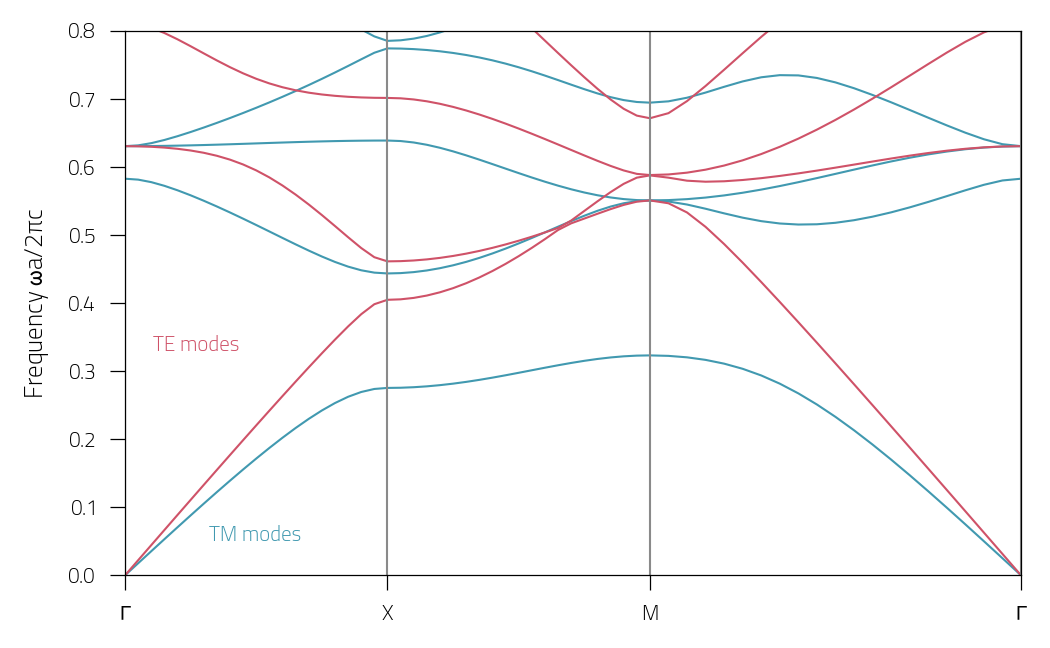
Band diagram of 2D photonic crystal

Calculation of the band diagram of a two-dimensional photonic crystal.

import matplotlib.pyplot as plt
import numpy as np

import protis as pt

pi = np.pi

Reference results are taken from [Joannopoulos2008] (Chapter 5 Fig. 2).

The structure is a square lattice of dielectric columns, with radius r and dielectric constant \(\varepsilon\). The material is invariant along the z direction and periodic along \(x\) and \(y\) with lattice constant \(a\). We will define the lattie using the class Lattice

a = 1
lattice = pt.Lattice([[a, 0], [0, a]], discretization=2**9)

Define the permittivity

epsilon = lattice.ones() * 1
rod = lattice.circle(center=(0.5, 0.5), radius=0.2)
epsilon[rod] = 8.9

We define here the wavevector path:

Gamma = (0, 0)
X = (pi / a, 0)
M = (pi / a, pi / a)
sym_points = [Gamma, X, M, Gamma]

Nb = 21
kpath = pt.init_bands(sym_points, Nb)

Calculate the band diagram:

sim = pt.Simulation(lattice, epsilon=epsilon, nh=100)

BD = {}
for polarization in ["TE", "TM"]:
    ev_band = []
    for kx, ky in kpath:
        sim.k = kx, ky
        sim.solve(polarization, vectors=False)
        ev_norma = sim.eigenvalues * a / (2 * pi)
        ev_band.append(ev_norma)
    BD[polarization] = ev_band
BD["TM"] = pt.backend.stack(BD["TM"]).real
BD["TE"] = pt.backend.stack(BD["TE"]).real

Plot the bands:

labels = ["$\Gamma$", "$X$", "$M$", "$\Gamma$"]


plt.figure()
plotTM = pt.plot_bands(sym_points, Nb, BD["TM"], color="#4199b0")
plotTE = pt.plot_bands(sym_points, Nb, BD["TE"], xtickslabels=labels, color="#cf5268")

plt.annotate("TM modes", (1, 0.05), c="#4199b0")
plt.annotate("TE modes", (0.33, 0.33), c="#cf5268")
plt.ylim(0, 0.8)
plt.ylabel(r"Frequency $\omega a/2\pi c$")
plt.tight_layout()

Estimated memory usage: 27 MB