Reduced Bloch mode expansion

Calculation of the band diagram of a two-dimensional photonic crystal.

import matplotlib.pyplot as plt
import numpy as np

import protis as pt

Reference results are taken from [Hussein2009].

a = 1
lattice = pt.Lattice([[a, 0], [0, a]], discretization=2**9)

Define the permittivity

epsilon = lattice.ones() * 1
hole = lattice.square((0.5, 0.5), 0.33)
epsilon[hole] = 11.4
mu = 1

We define here the wavevector path:

def k_space_path(Nb):
    K = np.linspace(0, np.pi / a, Nb)
    bands = np.zeros((3 * Nb - 3, 2))
    bands[:Nb, 0] = K
    bands[Nb : 2 * Nb, 0] = K[-1]
    bands[Nb : 2 * Nb - 1, 1] = K[1:]
    bands[2 * Nb - 1 : 3 * Nb - 3, 0] = bands[2 * Nb - 1 : 3 * Nb - 3, 1] = np.flipud(
        K
    )[1:-1]
    return bands, K

Full model:

def full_model(bands, nh=100):
    t0 = pt.tic()
    sim = pt.Simulation(lattice, epsilon=epsilon, mu=mu, nh=nh)
    BD = {}
    for polarization in ["TE", "TM"]:
        ev_band = []
        for kx, ky in bands:
            sim.k = kx, ky
            sim.solve(polarization, vectors=False)
            ev_norma = sim.eigenvalues * a / (2 * np.pi)
            ev_band.append(ev_norma)
        # append first value since this is the same point
        ev_band.append(ev_band[0])
        BD[polarization] = ev_band
    BD["TM"] = pt.backend.stack(BD["TM"]).real
    BD["TE"] = pt.backend.stack(BD["TE"]).real
    t_full = pt.toc(t0, verbose=False)
    return BD, t_full, sim

Reduced Bloch mode expansion

def rbme_model(bands, nh=100, Nmodel=2, N_RBME=8):
    t0 = pt.tic()
    sim = pt.Simulation(lattice, epsilon=epsilon, mu=mu, nh=nh)
    q = pt.pi / a
    if Nmodel == 2:
        bands_RBME = [(0, 0), (q, 0), (q, q)]
    elif Nmodel == 3:
        bands_RBME = [(0, 0), (q / 2, 0), (q, 0), (q, q / 2), (q, q), (q / 2, q / 2)]
    else:
        raise ValueError
    rbme = {
        polarization: sim.get_rbme_matrix(N_RBME, bands_RBME, polarization)
        for polarization in ["TE", "TM"]
    }
    BD_RBME = {}
    for polarization in ["TE", "TM"]:
        ev_band = []
        for kx, ky in bands:
            sim.k = kx, ky
            sim.solve(polarization, vectors=False, rbme=rbme[polarization])
            ev_norma = sim.eigenvalues * a / (2 * np.pi)
            ev_band.append(ev_norma)
        # append first value since this is the same point
        ev_band.append(ev_band[0])
        BD_RBME[polarization] = ev_band
    BD_RBME["TM"] = pt.backend.stack(BD_RBME["TM"]).real
    BD_RBME["TE"] = pt.backend.stack(BD_RBME["TE"]).real
    t_rbme = pt.toc(t0, verbose=False)
    return BD_RBME, t_rbme, sim


bands, K = k_space_path(Nb=49)
BD, t_full, sim_full = full_model(bands, nh=100)
BD_RBME, t_rbme, sim_rbme = rbme_model(bands, nh=100, Nmodel=2, N_RBME=8)
print(f"speedup = {t_full/t_rbme}")

speedup = 4.113342513115059

Plot the bands:

def k_space_path_plot(Nb, K):
    bands_plot = np.zeros(3 * Nb - 2)
    bands_plot[:Nb] = K
    bands_plot[Nb : 2 * Nb - 1] = K[-1] + K[1:]
    bands_plot[2 * Nb - 1 : 3 * Nb - 2] = 2 * K[-1] + 2**0.5 * K[1:]
    return bands_plot


bands_plot = k_space_path_plot(49, K)

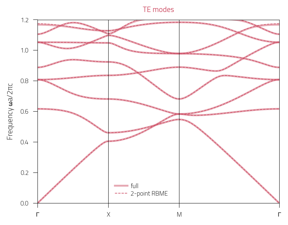
TE polarization:

plt.figure(figsize=(3.2, 2.5))
plotTE = plt.plot(bands_plot, BD["TE"], c="#cf5268", lw=1.5, alpha=0.5)
plotTE_RBME = plt.plot(bands_plot, BD_RBME["TE"], "--", c="#cf5268")
plt.ylim(0, 1.2)
plt.xlim(0, bands_plot[-1])
plt.xticks(
    [0, K[-1], 2 * K[-1], bands_plot[-1]], ["$\Gamma$", "$X$", "$M$", "$\Gamma$"]
)
plt.axvline(K[-1], c="k", lw=0.3)
plt.axvline(2 * K[-1], c="k", lw=0.3)
plt.ylabel(r"Frequency $\omega a/2\pi c$")
plt.legend([plotTE[0], plotTE_RBME[0]], ["full", "2-point RBME"], loc=(0.31, 0.02))
plt.title("TE modes", c="#cf5268")
plt.tight_layout()

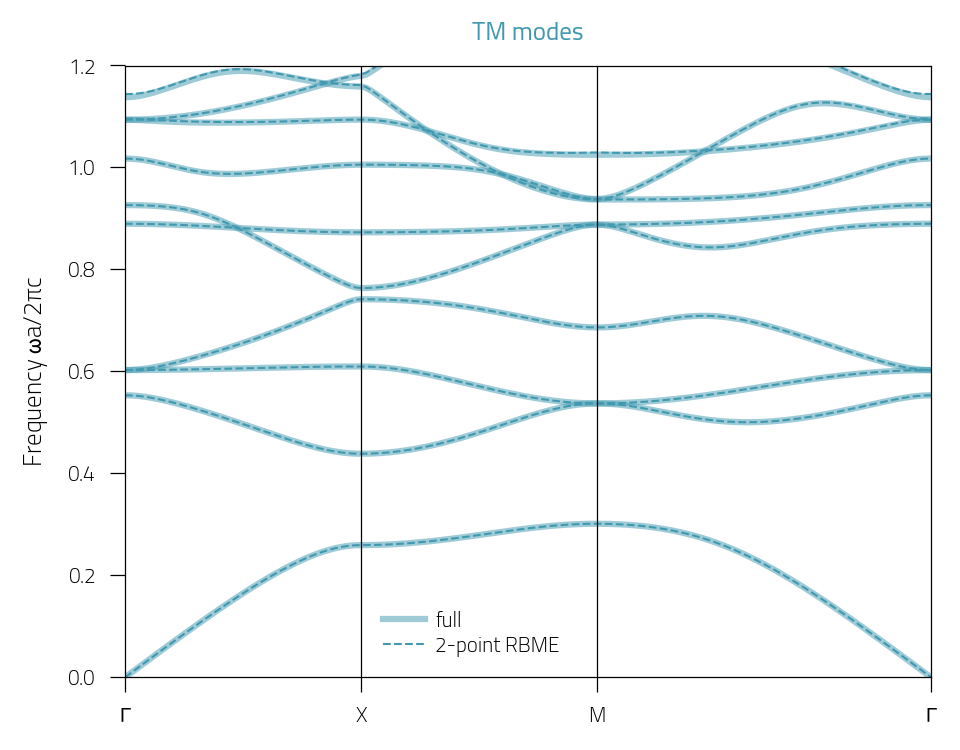
TM polarization:

plt.figure(figsize=(3.2, 2.5))
plotTM = plt.plot(bands_plot, BD["TM"], c="#4199b0", lw=1.5, alpha=0.5)
plotTM_RBME = plt.plot(bands_plot, BD_RBME["TM"], "--", c="#4199b0")
plt.ylim(0, 1.2)
plt.xlim(0, bands_plot[-1])
plt.xticks(
    [0, K[-1], 2 * K[-1], bands_plot[-1]], ["$\Gamma$", "$X$", "$M$", "$\Gamma$"]
)
plt.axvline(K[-1], c="k", lw=0.3)
plt.axvline(2 * K[-1], c="k", lw=0.3)
plt.ylabel(r"Frequency $\omega a/2\pi c$")
plt.legend([plotTM[0], plotTM_RBME[0]], ["full", "2-point RBME"], loc=(0.31, 0.02))
plt.title("TM modes", c="#4199b0")
plt.tight_layout()

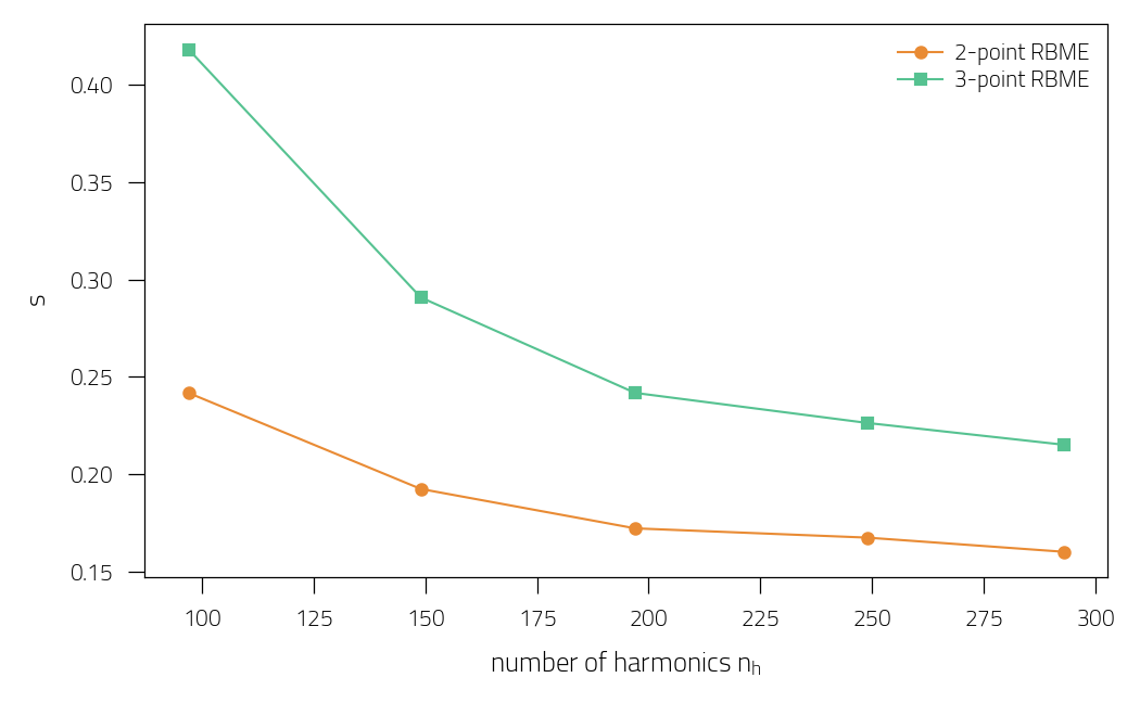
Performances with number of harmonics

bands, K = k_space_path(49)
NH = np.arange(100, 350, 50)
actual_nh = []
s2 = []
s3 = []
for nh in NH:
    BD, t_full, sim_full = full_model(bands, nh=nh)
    BD_RBME2, t_rbme2, sim_rbme2 = rbme_model(bands, nh=nh, Nmodel=2, N_RBME=8)
    BD_RBME3, t_rbme3, sim_rbme3 = rbme_model(bands, nh=nh, Nmodel=3, N_RBME=8)
    actual_nh.append(sim_full.nh)
    s2.append(t_rbme2 / t_full)
    s3.append(t_rbme3 / t_full)


plt.figure()
plt.plot(actual_nh, s2, "o-", c="#e98b34", label="2-point RBME")
plt.plot(actual_nh, s3, "s-", c="#56c291", label="3-point RBME")
plt.xlabel(r"number of harmonics $n_h$")
plt.ylabel(r"$s$")
plt.legend()
plt.tight_layout()

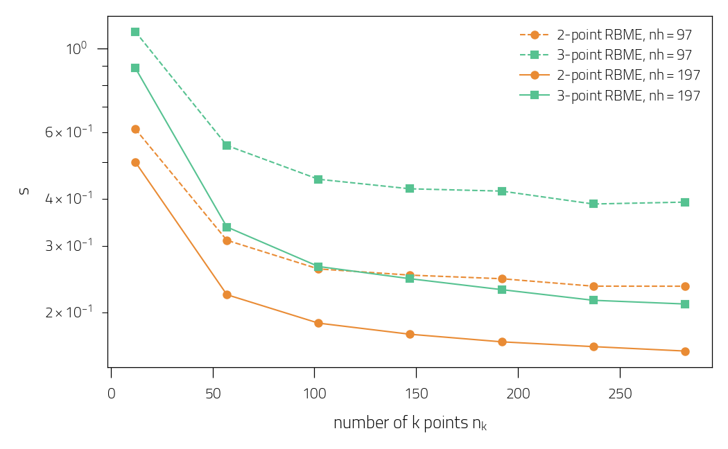
Performances with number of k-space points

result = {}
NH = [100, 200]
num_ks = np.arange(5, 100, 15)
for nh in NH:
    actual_nh = []
    nk = []
    s2 = []
    s3 = []
    for Nb in num_ks:
        bands, K = k_space_path(Nb)
        nk.append(len(bands))
        BD, t_full, sim_full = full_model(bands, nh=nh)
        BD_RBME2, t_rbme2, sim_rbme2 = rbme_model(bands, nh=nh, Nmodel=2, N_RBME=8)
        BD_RBME3, t_rbme3, sim_rbme3 = rbme_model(bands, nh=nh, Nmodel=3, N_RBME=8)
        actual_nh.append(sim_full.nh)
        s2.append(t_rbme2 / t_full)
        s3.append(t_rbme3 / t_full)
    result[nh] = dict(s2=s2, s3=s3, actual_nh=actual_nh)


plt.figure()
plt.plot(
    nk,
    result[NH[0]]["s2"],
    "o--",
    c="#e98b34",
    label=rf"2-point RBME, $nh={result[NH[0]]['actual_nh'][0]}$",
)
plt.plot(
    nk,
    result[NH[0]]["s3"],
    "s--",
    c="#56c291",
    label=rf"3-point RBME, $nh={result[NH[0]]['actual_nh'][0]}$",
)
plt.plot(
    nk,
    result[NH[1]]["s2"],
    "o-",
    c="#e98b34",
    label=rf"2-point RBME, $nh={result[NH[1]]['actual_nh'][0]}$",
)
plt.plot(
    nk,
    result[NH[1]]["s3"],
    "s-",
    c="#56c291",
    label=rf"3-point RBME, $nh={result[NH[1]]['actual_nh'][0]}$",
)
plt.xlabel(r"number of k points $n_k$")
plt.ylabel(r"$s$")
plt.legend()
plt.yscale("log")
plt.tight_layout()

Estimated memory usage: 13 MB